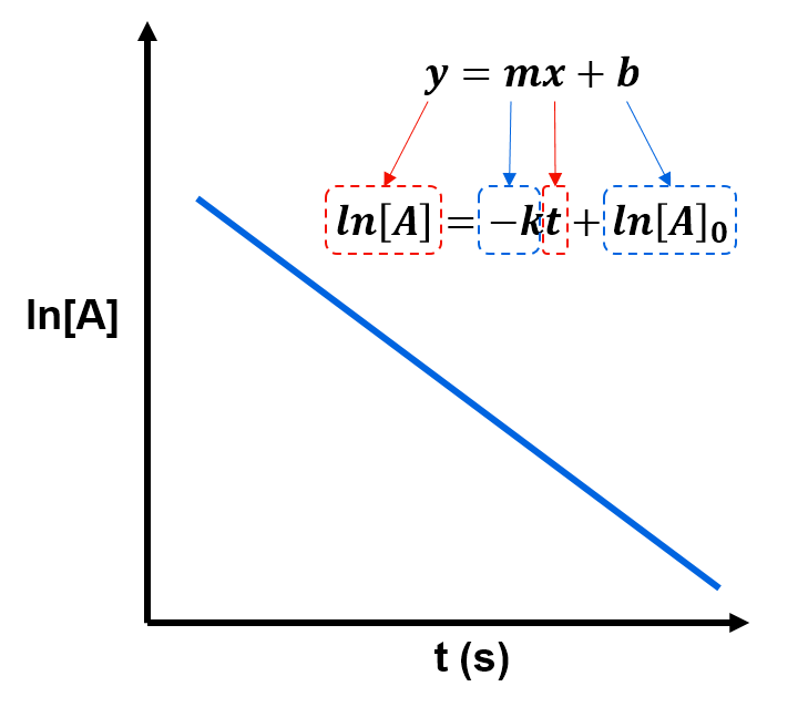
- For a reaction that is first order in reactant A, a plot of ln[A] vs time (t) gives a straight line with equation
such that the slope is -k and the y-intercept is b=ln[A]0
- The concentration of A ([A]) for a first order reaction can be caluculated for any time (t) using the equation
So far we have studied how the rate of a reaction relates to (1) the rate of change of the concentration of each reactant/product and (2) the concentration of each reactant. For example, the rate of the generic elementary reaction
is
(Equation 1).
In this section, we will derive an equation that can describe the concentration of a reactant at a particular time. This derivation will require a basic understanding of integral calculus. If you're not familiar with integral calculus, please review the expandable section below before working through the derivation.
Review: Expand this section for a brief overview of integral calculus.
In section 1.2 we used derivatives to describe the rate (slope) of a concentration versus time graph. We don't yet have an equation, though, to describe a concentration versus time graph.
Consider an example where the concentration of reactant A decreases linearly over time, as shown by the left graph below.
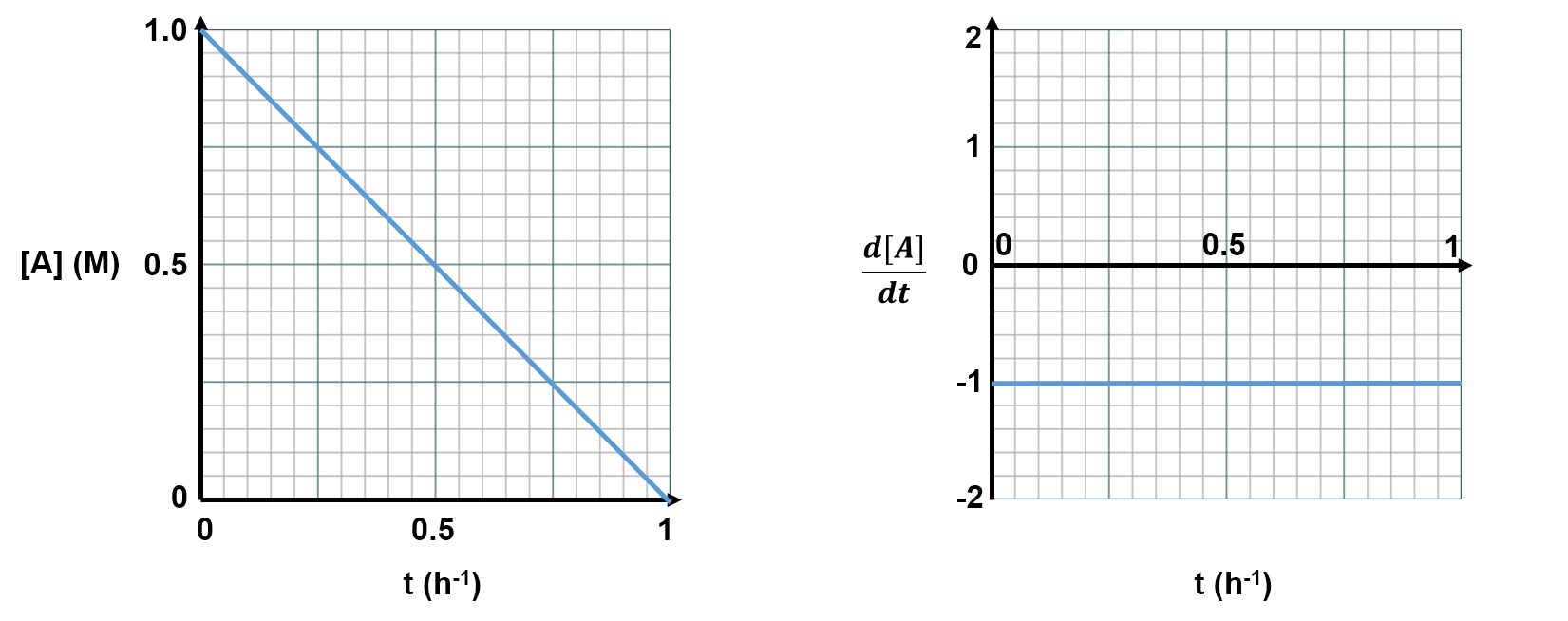
This is a linear plot, so the slope () is the same at every time, t. Thus, a plot of the derivative (slope;
) versus time, t, would look like the plot on the right. This right plot shows how [A] is changing at each time, t. Imagine if we wanted to use the right graph to get back to the left graph. The y-axis of the right graph tells us how much the concentration changes over a given time. If we multiplied
(the y-value) by
(the x-value), then we would get the total change in concentration over this time period (the '
' component would cancel to leave the change in [A] only). This is analagous to finding the area between the graph and the x-axis. For example, from time t=0s to t=0.5s, the area between the plotted line and the x axis is shown by the green box below
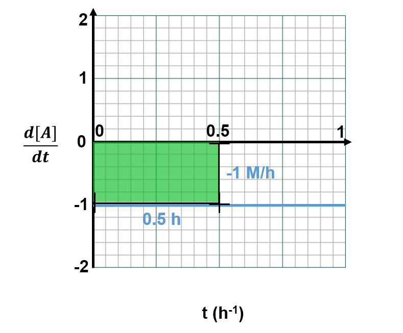
and is thus
.
This exactly matches the top left graph, which shows that from time t=0h to t=0.5h, the concentration of A has dropped from 1.0 M to 0.5 M (i.e., decreased by 0.5 M). When the plots are linear it's simple to do these conversions. When plots are curved, the mathematics is more complex, but the concept is the same: the area under a the curve of a versus
graph from 0 to time t will always give the total change in [A] up to time t. Mathematically, this equates to taking the antiderivative ('undoing the derivative'), which gets us from
versus
back to
versus
. This process of finding the area under a curve is called integration. You will be expected to be able to reproduce two integrals in this course (one introduced below and the second on the next page). Integral calculus is not a prerequisite for this course, so you will not be asked to evaluate any unfamiliar integrals.
Let's find an equation for [A] vs time for the simple, first order elementary reaction
with rate
(Equation 1).
Equation 1 is called a differential equation because it includes a derivative. Since we can isolate the components that relate to concentration on the left side from the components that relate to time on the right side, this is a separable differential equation which can be written as
.
Integrating the left side of the equation from the concentration at time ,
, to the concentration at time
,
, and integrating the right side from time
to time
gives
Integration help: What does this mean?
The symbol indicates an integral. Conceptually, this means that we are determining the area under the curve (between the plotted line and the x-axis) for our indicated functions:
on the left and
on the right. The integrals here have labels at the bottom (
and 0) and top (
and
), which indicates a definite integral. This means that on the left we are finding the area underneath the function
between
and
and on the right we are finding the area underneath the function
between
and
.
Solving this integral gives
Integration help: What does this mean?
Here we have shown that the integral of is
and that the integral of
is
. You are not expected to know why these are the integral functions. You should, though, be able to reproduce this result. You will not be asked for any unfamiliar integrals in CHEM 123, since integral calculus is not a prerequisite. The area under the curve between the indicated points (
and
on the left;
and
on the right) has not yet been evaluated, though. The part that states
should be read "evaluated from to
" and means that the value of the integrated function,
, when
should be subtracted from the value of the integrated function when
such that
.
Analogously, on the right side of the equation
.
Rearranging this result slightly gives
which is also often written as
(Equation 2)
where it's understood that means the concentration of A at time t. This rearranged version of the integrated rate law is helpful because it is in linear form where
and
. By analogy with the generic linear equation
, this means that a plot of
versus
gives a straight line with slope
and y-intercept
. That is, we can use such a linear plot to measure the rate constant,
, and the initial concentration,
.
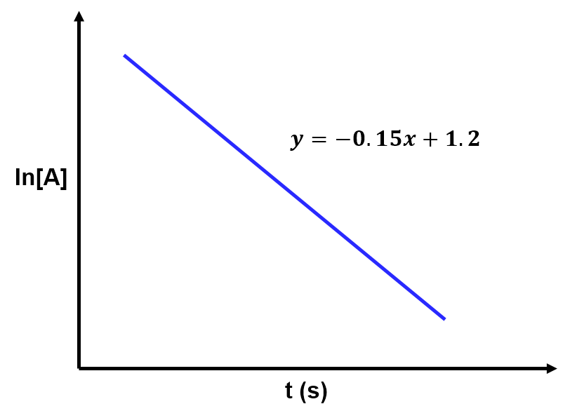
View solution:
The slope of the line relates to the rate constant by . Based on the given best fit line,
and thus the rate constant is
Solving Equation 2 for shows directly how
changes over time
(Equation 3).
That is, in a first order reaction the concentration of the reactant decreases exponentially over time. Equation 3 is useful for determining the concentration of reactant A at any time after the reaction starts.
Interactive:
Need help getting started? Check the example in the content above.